As of 2025, businesses continue to face a major disconnect between data collection and actual insight. According to recent research, 68% of enterprise data still goes unused in analytics workflows. This isn’t due to lack of access—it’s because the data often lives in unstructured, all-in-one tables that aren’t fit for analysis at scale.
Compounding the issue, 71% of organizations now report that their business intelligence tools struggle to scale with growing data, and 76% say slow or cluttered dashboards are affecting decision-making. The root cause? Poor data modeling. Without clear fact and dimension separation, even modern BI tools can’t perform efficiently.
Addressing these challenges, Microsoft Build 2025 introduced significant enhancements to Power BI and unveiled Microsoft Fabric, a unified data platform designed to streamline data management and analytics. These advancements aim to empower organizations to transform raw data into structured, insightful information efficiently.
That’s why, in this blog, we focus on one of the most practical and powerful modeling approaches available in Power BI—creating a Star Schema from a Single Table using Power Query. We’ll show you how to take a flat table and break it into a clean, scalable data model, step by step, using native Power BI tools.
Step 1: Understanding the Dataset to Create Star Schema
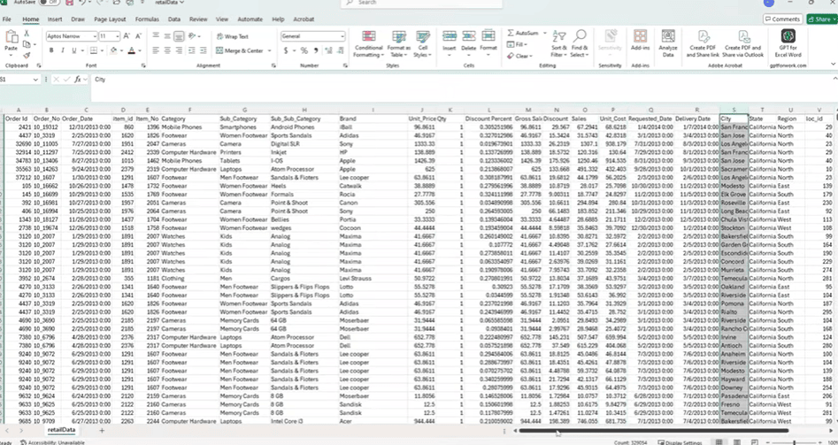
Many business datasets are delivered as flat tables—single sheets containing a mix of transactional and descriptive data. These tables often include sales values, product details, customer information, payment methods, and geographic fields, all combined in one structure.
While this format is easy to work with initially, it creates several issues in Power BI. Mixing repeated descriptive fields with transactional data leads to larger file sizes, unnecessary redundancy, and slower performance. It also complicates relationship management and limits the flexibility of the data model.
To resolve this, the data needs to be restructured into a star schema. In this approach:
- A fact table holds transactional data such as sales, quantity, cost, and discount.
- Dimension tables store descriptive attributes like product categories, regions, or payment methods.
The dataset used in this example contains:
- Sales details: Order ID, Order Date, Unit Price, Quantity, Discount
- Product attributes: Item ID, Category, Subcategory, Brand
- Geography: City, State, Region, Location ID
- Business descriptors: Payment Method, Order Type, Customer ID
This structure makes it suitable for building a star schema, which improves performance and supports scalable reporting in Power BI. In the next steps, Power Query will be used to transform this flat table into a clean, relational model.
Step 2: Loading the Flat File into Power BI Using Power Query
To begin building the star schema, the first step is importing the dataset into Power BI using Power Query. Here’s how the process works, broken down for clarity.
1. Open Power BI and Get the Data
- Launch Power BI Desktop.
- Go to the Home tab and select Get Data.
- Choose your data source:
- Use Web if the file is hosted online (e.g. a GitHub or Dropbox link).
- Use Excel if it’s stored locally.
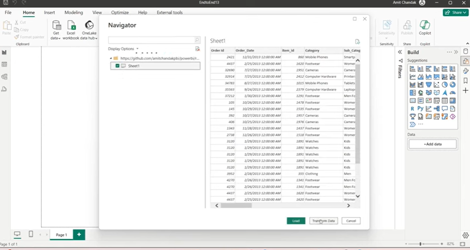
2. Select the Table
- After connecting, Power BI will show a list of available sheets or tables.
- Select the one that contains the raw data.
- Do not load the data yet—click Transform Data instead.
- This opens the Power Query Editor.
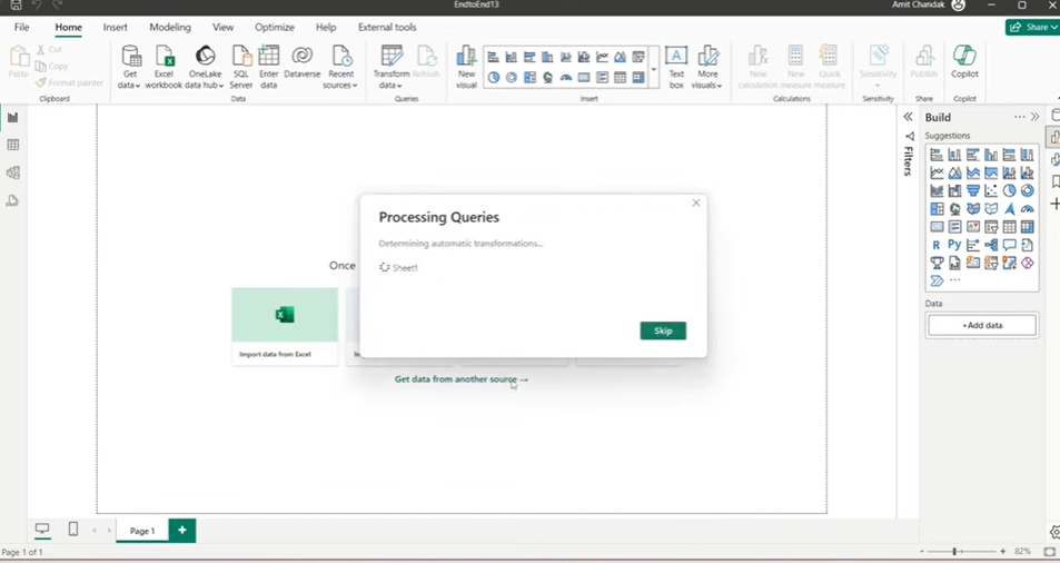
3. Review the Table Structure
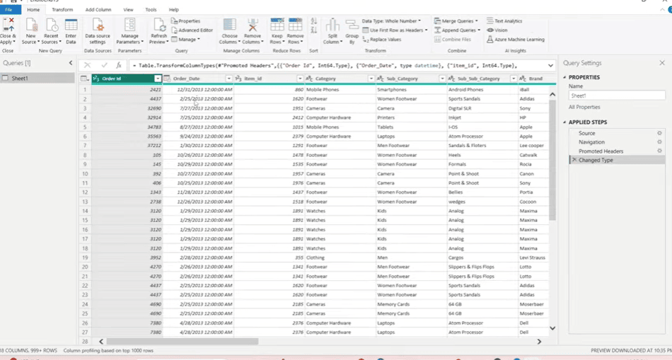
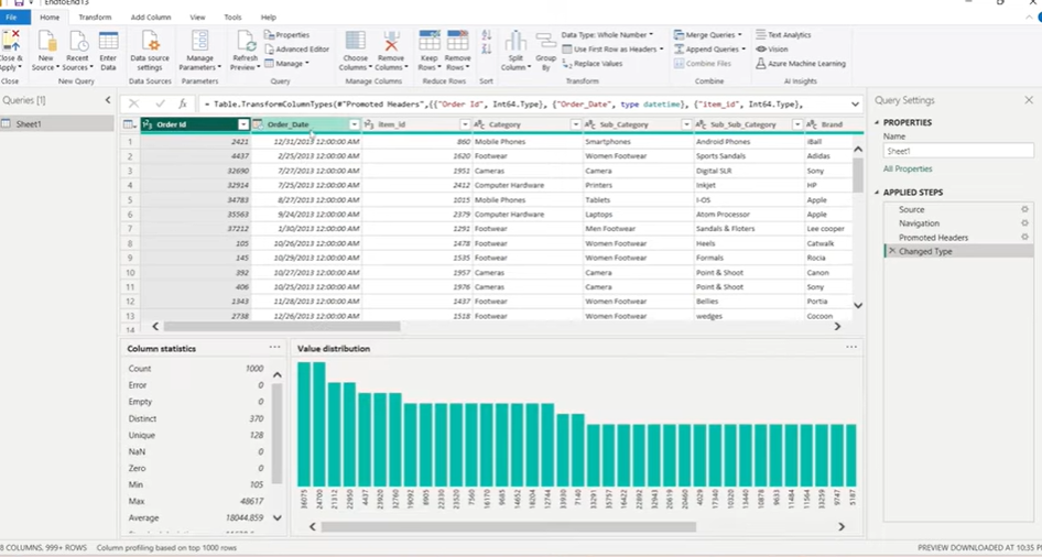
The table should now be open in Power Query. It contains:
- Transactional fields – Order ID, Order Date, Unit Price, Quantity, Discounts
- Product attributes – Item ID, Category, Subcategory, Brand
- Geographic fields – City, State, Region, Location ID
- Business fields – Payment Method, Order Type, Customer ID
This flat structure includes both descriptive fields and numeric values. It’s not optimized for reporting but provides everything we need to build a structured model.
4. Why Use Power Query
Power Query lets you:
- Split one table into many (facts and dimensions)
- Remove duplicates
- Create index columns
- Merge and join tables
- Apply all transformations before the data reaches the model
This gives you full control over how the data is shaped and ensures the final model in Power BI is clean, fast, and reliable.
Step 3: Creating Dimension Tables for Power BI Star Schema
Once the data is loaded into Power Query, the next step is to break the flat table into dimension tables. These dimensions will store repeated descriptive values such as product info, locations, and payment types. This improves performance and helps create a proper star schema.
We’ll create dimension tables using the Reference option in Power Query.
1. Use “Reference” Instead of “Duplicate”
In Power Query, you can either:
- Duplicate a table – creates a separate copy with no link to the original
- Reference a table – creates a linked version that shares the data source
Always use Reference when building dimensions. It loads data only once and reduces memory usage.
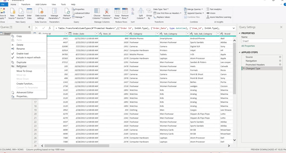
To create a reference:
- Right-click the main table
- Select Reference
- A new query will be created, linked to the original
2. Build the Product (Item) Dimension
This table contains product-related attributes.
Steps:
- Reference the main table
- Select the following columns:
- Item ID
- Category
- Subcategory
- Sub-subcategory
- Brand
- Right-click → Remove Other Columns
- Use Remove Duplicates to ensure uniqueness
- Go to View > Column Distribution to confirm Item ID is unique
- Rename this query to Item
This becomes your Item Dimension.
3. Build the Geography Dimension
Next, we create a table with geographic data.
Steps:
- Reference the main table
- Select:
- City
- State
- Location ID
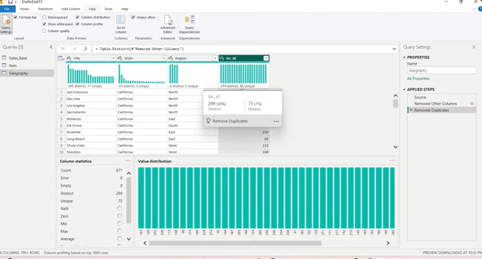
- Remove other columns
- If Region causes duplication, remove it
- Use Remove Duplicates
- Check column distribution to ensure Location ID is unique
- Rename the query to Geography
4. Build Single-Column Dimensions (Optional but Recommended)
Some fields like Payment Method, Order Type, or Region are standalone values that still deserve their own dimensions.
Steps (for each field):
- Reference the main table
- Keep only one column (e.g. Payment Method)
- Remove duplicates
- Add an Index Column (starting from 1) to act as a unique key
- Rename the query to match the column (e.g. Payment Method)
This approach ensures even small lookup tables are normalized.
Step 4: Building the Fact Table for the Star Schema Using Power Query
With the dimension tables ready, the next step is to build the fact table. This table holds the transactional data—sales amounts, quantities, costs—and connects to each dimension using ID columns.
We’ll build the fact table by referencing the base table and merging it with the dimension tables.
1. Start from the Base Table
- Go back to the main query (the original flat table)
- Rename it to something like Sales Base
- Do not make any changes to this query—it will serve only as a source
2. Create a Reference for the Fact Table
- Right-click Sales Base
- Choose Reference
- Rename the new query to Sales Fact
- This will become your main fact table
3. Merge Dimension Tables
You’ll now join each dimension to the fact table to bring in the related ID fields.
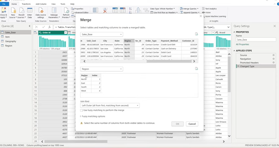
Example: Merge Geography
- In Sales Fact, go to Home > Merge Queries
- Select the Region column in both tables (Sales Fact and Geography)
- Use Left Outer Join
- Click OK
- Expand the merged column
- Select only the index or ID column (e.g. Region ID)
- Rename the column properly
Repeat the same steps to merge:
- Item table using Item ID
- Payment Method table using Payment Method
- Order Type table if needed
- Any other single-column dimensions you’ve created
4. Finalize the Fact Table
Once all merges are done:
- Keep only necessary fields
- Ensure all dimension IDs are present
- Confirm numeric fields like:
- Unit Price
- Quantity
- Gross Sales
- Discount
- Net Sales
- Optionally, create calculated columns (e.g. Gross Amount = Quantity * Unit Price)
Now the fact table is complete, with proper keys linking it to each dimension.
5. Apply the Changes
- Click Close & Apply in Power BI
- Power BI will load all the tables into the data model
- Loading order matters—dimension tables will load first, followed by the fact table
Microsoft Fabric vs Power BI: How They Differ and Which One You Need
An in-depth comparison of Microsoft Fabric and Power BI, explaining their differences, use cases, and how to choose the right solution for your data and analytics needs.
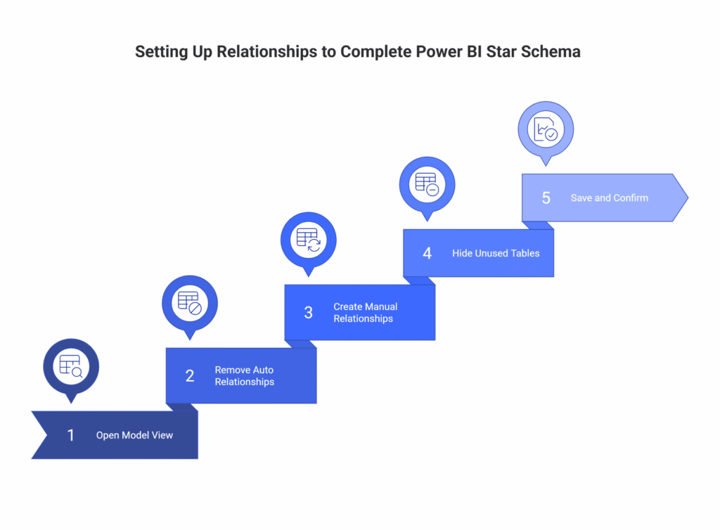
Step 5: Setting Up Relationships to Complete Power BI Star Schema
Once the fact and dimension tables are loaded into Power BI, the final step is to define relationships between them. This creates the actual star schema—a central fact table connected to multiple dimension tables.
Power BI may auto-detect relationships, but it’s best to set them manually to ensure accuracy.
1. Open Model View
- In Power BI Desktop, switch to the Model view from the left sidebar
- You’ll see all your tables laid out as blocks
- If Power BI created relationships automatically, review them carefully
2. Remove Incorrect Auto Relationships
- Select and delete any automatically created relationships
- These are often based on column name matches and may not reflect the actual keys you want to use
- It’s better to define all joins manually
3. Create Manual Relationships
For each dimension, connect its key column to the matching column in the fact table.
Examples:
- Item[Item ID] → Sales Fact[Item ID]
- Geography[Location ID] → Sales Fact[Location ID]
- Payment Method[Payment Method ID] → Sales Fact[Payment Method ID]
- Region[Region ID] → Sales Fact[Region ID] (if applicable)
Settings to use:
- Cardinality: Many-to-One (fact → dimension)
- Cross Filter Direction: Single
Power BI should detect these settings correctly but always double-check.
4. Hide Unused Tables (Optional)
To keep the model clean:
- Right-click on Sales Base (the untouched reference table)
- Select Hide in Report View
- This keeps it in the background for queries but removes clutter from visuals
5. Save and Confirm
- At this point, your star schema is complete
- Save your file
- Test visuals to confirm that relationships work as expected
With all joins defined, Power BI can now read the model efficiently. This improves performance, reduces redundancy, and simplifies visualizations and DAX logic.
Step 6: Apply and Load Star Schema Model in Power BI
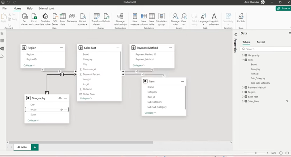
With all tables loaded and cleaned, the final task is to connect the fact table to the dimension tables. This is done in Power BI’s Model View, where you define relationships and complete the star schema.
1. Hide the Base Table (Optional)
The original flat table, now renamed as Sales Base, is no longer needed for reports. To reduce clutter:
- Right-click on Sales Base
- Select Hide in Report View
- This keeps the query for reference but removes it from visual-level tools
2. Define Relationships Manually
Power BI may try to auto-detect joins, but it’s best to create them yourself. Each dimension should connect to the fact table using its ID column.
Set up these joins:
- Sales Fact[Item ID] → Item[Item ID]
- Sales Fact[Location ID] → Geography[Location ID]
- Sales Fact[Payment Method ID] → Payment Method[Payment Method ID]
- Sales Fact[Region ID] → Region[Region ID] (if a Region table was created)
3. Set Relationship Properties
For each join:
- Cardinality: Many-to-One (the fact table has repeated values, the dimension doesn’t)
- Cross Filter Direction: Single (from dimension to fact)
These settings ensure your model behaves predictably in visuals and DAX calculations.
Once relationships are in place, your star schema is complete. The model is now ready for building fast, scalable, and reliable reports in Power BI.
Real-World Use Case: Applying Star Schema Using Power Query in Power BI
Use Case 1: E-commerce Sales Dashboard
Scenario:
An online retail company stores monthly transaction data in a centralized system. The export includes:
- Order ID, Order Date, Product Name, Category, Subcategory
- Quantity, Unit Price, Discount, Total Amount
- Payment Method, Shipping City, Customer ID
All of this is in a single flat Excel or CSV file shared with the BI team.
Problem with the Flat Table:
- Every row repeats product and category info
- City names are spelled inconsistently (e.g. “New York”, “NYC”, “new york”)
- Adding a new metric or dimension becomes harder over time
- Reports get slower as data grows
Star Schema Fix:
Split the data into:
- Fact_Sales: Order-level transactional data (Order ID, Quantity, Unit Price, Discount, Total)
- Dim_Product: Product ID, Product Name, Category, Subcategory
- Dim_Payment: Payment Method, with an assigned PaymentMethodID
- Dim_Geography: City, State, Region, Location ID
Example Power Query Steps (Product Table):

Business Impact:
- Clean slicers for Category or Payment Method
- Reports like “Top-Selling Products by Region” load instantly
- Easy to add measures like Gross Margin or Average Discount
- Can use Calendar Table and DATEADD() for YTD, MTD, or LY analysis
Use Case 2: Financial Performance Dashboard for a Services Company
Scenario:
A consulting firm tracks billing data across projects. Their Excel report contains:
- Invoice ID, Invoice Date, Client Name, Client Region, Service Type
- Consultant Name, Billing Rate, Hours Worked, Total Billed
The data is flat and includes many repeated names and service types.
Problem with the Flat Table:
- Every invoice row repeats client and service info
- Changing a client region requires updating many rows
- Complex filters (e.g., all hours billed for a certain service in a region) are slow and unreliable
Star Schema Fix:
Split the data into:
- Fact_Billing: Invoice ID, Consultant ID, Service ID, Client ID, Billing Rate, Hours, Total
- Dim_Client: Client ID, Client Name, Region
- Dim_Service: Service ID, Service Name, Type
- Dim_Consultant: Consultant ID, Name, Department
Example Measure in Power BI:


Business Impact:
- Analysts can easily slice by service, region, or consultant
- Drill-throughs to see billing by client or department become fast and reliable
- New service types can be added without touching historical data
- Regional managers get dashboards filtered to their territory with row-level security
These examples help highlight why star schema isn’t just a “best practice”—it’s the difference between a slow, fragile report and a robust analytics solution that scales.
Why Kanerika is Your #1 Choice for Data Modernization Services
As a leading provider of data and AI solutions, Kanerika recognizes the need for businesses to transition from legacy systems to modern data platforms. Upgrading outdated infrastructure enhances data accessibility, improves reporting accuracy, enables real-time insights, and lowers maintenance costs. With modern platforms, businesses can harness advanced analytics, cloud scalability, and AI-powered decision-making to stay ahead in a competitive landscape.
However, manual migration processes can be complex, time-intensive, and prone to errors, often disrupting critical business operations. Even a minor mistake in data mapping or transformation can lead to inconsistencies, historical data loss, or extended system downtime.
To address these challenges, Kanerika has developed custom automation solutions that streamline migrations across multiple platforms with precision and efficiency. Our automated tools ensure seamless transitions from SSRS to Power BI, SSIS and SSAS to Fabric, Informatica to Talend/DBT, and Tableau to Power BI, minimizing manual effort while preserving data integrity.
Partner with Kanerika for a seamless, automated, and risk-free data modernization experience.
Take Your Business to the Next Level with Innovative Power BI Solutions!
Partner with Kanerika today.
FAQs
What is the difference between star schema and wide table?
Wide Tables are more inflexible to change and are harder to maintain than the star schema. If the number of data sources increases, the whole table must be rebuilt. It also doesn’t handle changes in dimensions well, unlike star schema that can capture both the latest values and values at any given point in time.
What are the two types of tables in a star schema known?
Fact tables and dimension tables
A star schema has a single fact table in the center, containing business “facts” (like transaction amounts and quantities). The fact table connects to multiple other dimension tables along “dimensions” like time, or product.
Can you have multiple fact tables in a star schema?
The first step to handle multiple fact tables in a star schema is to identify the grain or level of detail of each fact table. The grain determines the key attributes that uniquely identify each row in the fact table, such as transaction ID, order ID, or invoice ID.


